From Spectrum to RGB Color - A practical protocol
Before starting, converting a spectrum to a RGB color is a very complicated process which involve human physiology, perception, technological limits, and international standards. There is a lot of theory behind it. I am no expert in this field, and what follows are just some practices that looks like they are working for me. Any comment or improvement is welcome!
One information that is possible to extract from an emission spectrum is the perceived color. Everybody knows that at different wavelengths correspond different colors of the rainbow: violet at 380–450nm, blue at 450–495nm, green at 495–570 nm, yellow at 570–590 nm, orange at 590–620 nm, and red at 620–750nm.

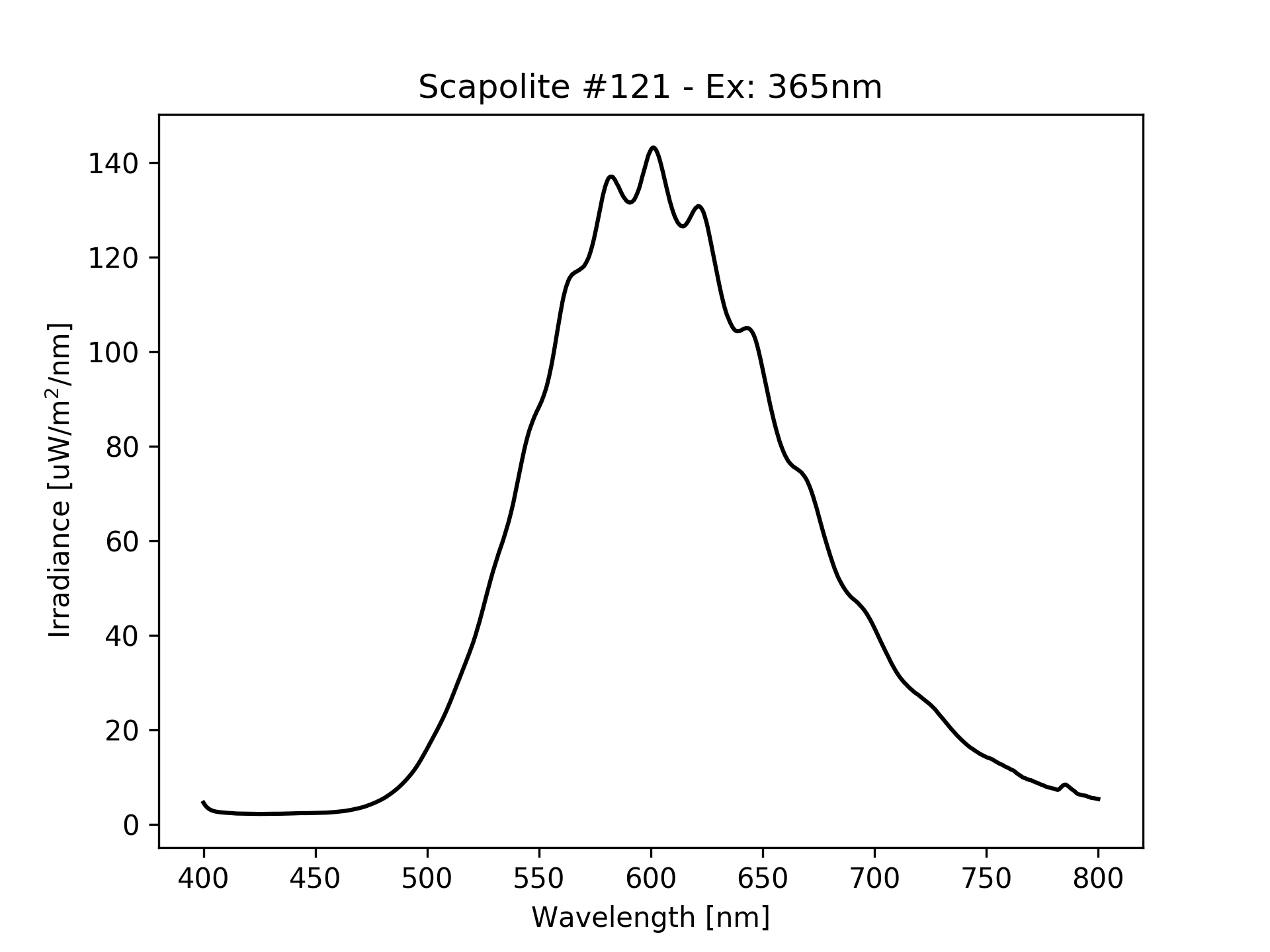
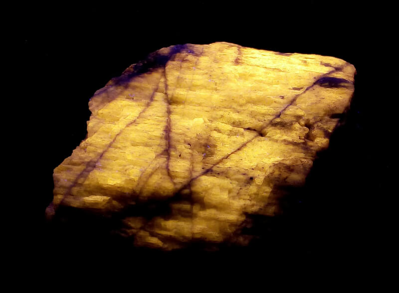
If the emission spectrum would be composed of just one peak in one of these regions, the perceived color would be very simple to identify. In most cases though, the spectrum is composed by a number of peaks, some high and thin, some low and spread, often overlapped. What to do then? For example, the following is the fluorescence spectrum of a mineral (scapolite from Canada). The spectrum is composed by a broad band between 500nm (bright green) and 750nm (deep red), with few smaller peaks in between. What color is this?
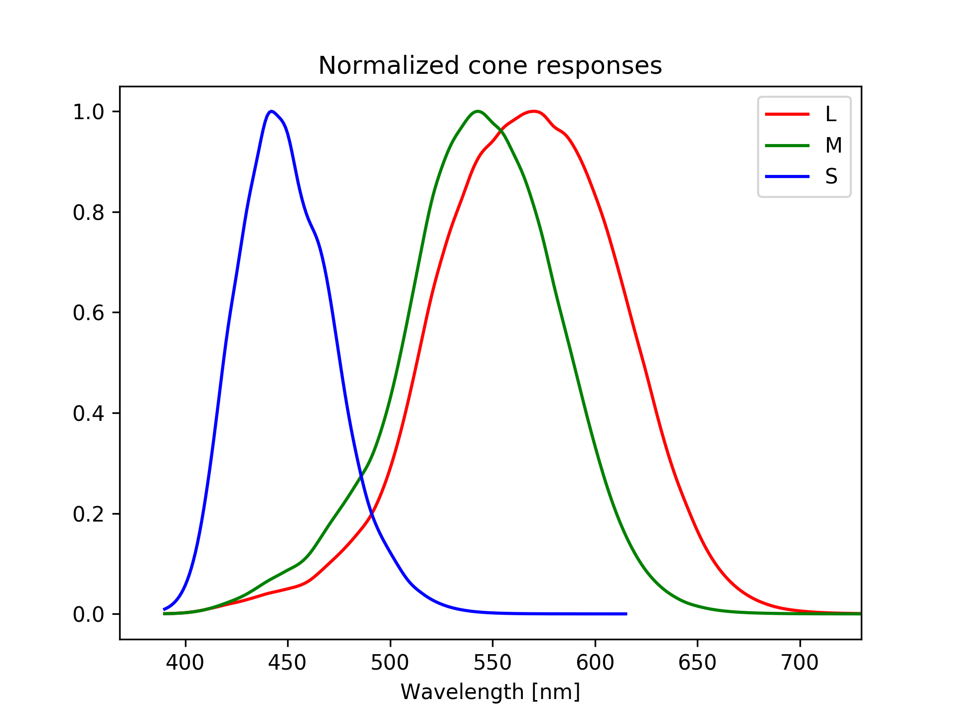
Human perceive colors thanks to the presence in the eye of three different cone cells (L, M, and S), each sensitive to a different range of wavelengths. When light enters the eye, the cones get stimulated differently based on the spectrum of that light. Then the three different stimuli from the three types of cone cells are put together to form the perceived color. What we can do is to reproduce this process, trying to simulate how a spectrum stimulates the three types of cone cells and then how this is perceived, or interpreted, by humans.
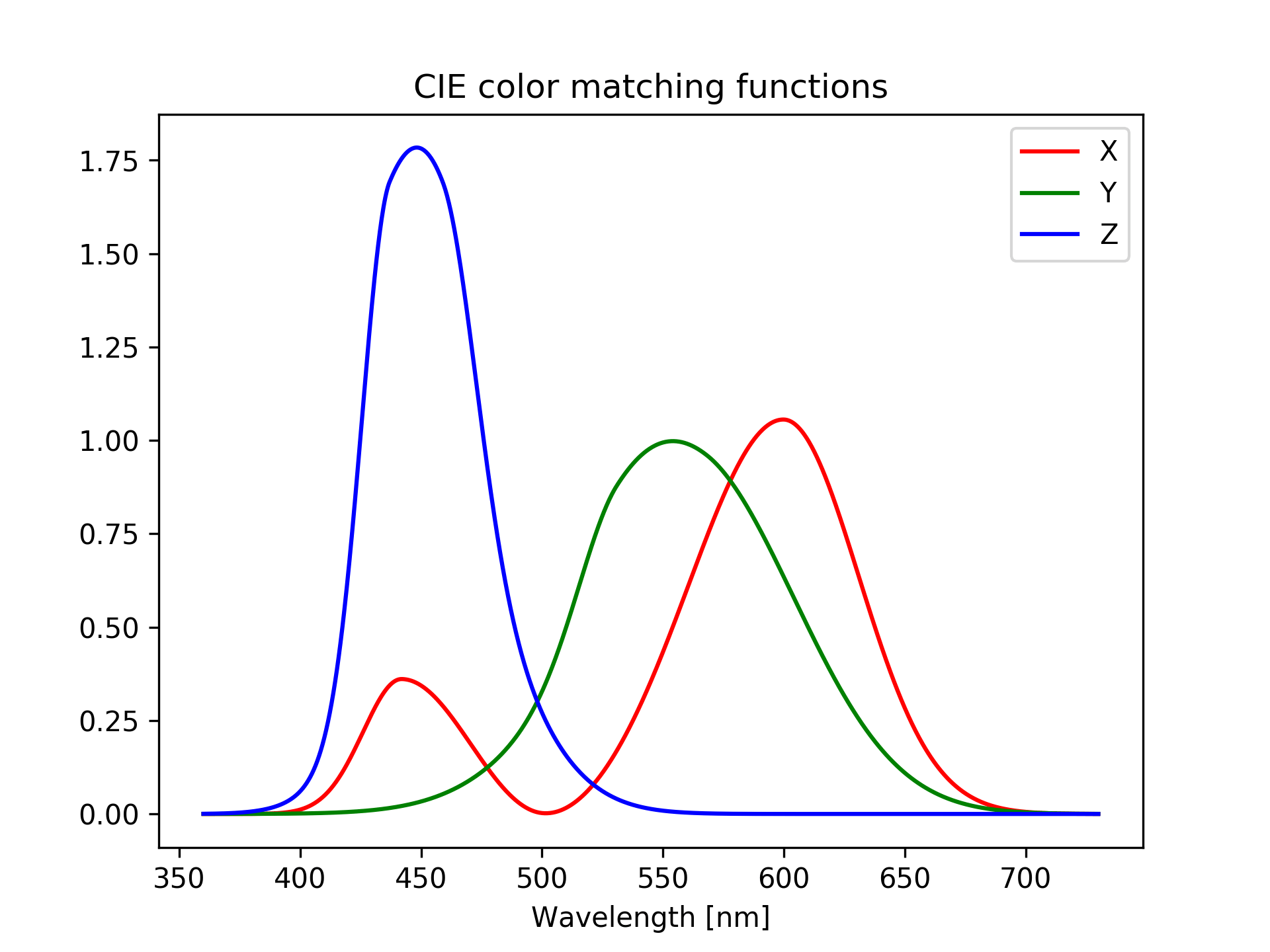
Working directly with a color space defined by the cone responses is, unfortunately, not the best solution. Long story short, the International Commission on Illumination (CIE) developed in 1931 a set of “color matching functions” for a “standard observer”. These are three functions that, similarly to the three cone cells, respond, or “get stimulated”, differently from different wavelengths. By comparing the spectrum with the three color matching functions, three values X, Y and Z are calculated. These define a color space, and we could happily stop here.
In a more mathematical form, the X, Y and Z values are computed as integral of the product between the spectrum and the three color matching functions. Calling the spectrum \(S(\lambda)\), where \(\lambda\) is the wavelength, and the matching functions \(\bar x(\lambda)\), \(\bar y(\lambda)\) and \(\bar z(\lambda)\), the XYZ values are computed as
\[ X = \int S(\lambda) \bar x(\lambda) d\lambda \approx \sum_i S(\lambda_i) \bar x(\lambda_i) \]
\[ Y = \int S(\lambda) \bar y(\lambda) d\lambda \approx \sum_i S(\lambda_i) \bar y(\lambda_i) \]
\[ Z = \int S(\lambda) \bar z(\lambda) d\lambda \approx \sum_i S(\lambda_i) \bar z(\lambda_i) \]
Given the arbitrary scale of the spectrum, it is nice at this point normalize the XYZ values such that their sum is one. Writing the integration and normalization steps into code we get:
def spectrum2xyz(S):
    X = np.sum(S*xbar)
    Y = np.sum(S*ybar)
    Z = np.sum(S*zbar)
    XYZ = X+Y+Z
    X /= XYZ
    Y /= XYZ
    Z /= XYZ
    return X, Y, Z
(note: sum(S*xbar) is a vector operation: multiply the i-th element of S with the i-th element of xbar and sum all the results.)
A last note on this point, the three color matching functions were defined in the 1931 numerically. Nowadays analytical approximations are available, which are much simpler to use. Here one:
def CIE_xyz_fit(wavel):
    """
        Simple Analytic Approximations to the CIE XYZ Color Matching Functions
        Chris Wyman, Peter-Pike Sloan, and Peter Shirley
        Journal of Computer Graphics Techniques, Vol. 2, No. 2, 2013
        http://jcgt.org/published/0002/02/01/
    """
    def xFit_1931(wave):
        t1 = (wave-442.0) * (0.0624 if (wave<442.0) else 0.0374)
        t2 = (wave-599.8) * (0.0264 if (wave<599.8) else 0.0323)
        t3 = (wave-501.1) * (0.0490 if (wave<501.1) else 0.0382)
        return 0.362*math.exp(-0.5*t1*t1) + 1.056*math.exp(-0.5*t2*t2) - 0.065*math.exp(-0.5*t3*t3)
    def yFit_1931(wave):
        t1 = (wave-568.8) * (0.0213 if (wave<568.8) else 0.0247)
        t2 = (wave-530.9) * (0.0613 if (wave<530.9) else 0.0322)
        return 0.821*math.exp(-0.5*t1*t1) + 0.286*math.exp(-0.5*t2*t2)
    def zFit_1931(wave):
        t1 = (wave-437.0)*(0.0845 if (wave<437.0) else 0.0278)
        t2 = (wave-459.0)*(0.0385 if (wave<459.0) else 0.0725)
        return 1.217*math.exp(-0.5*t1*t1) + 0.681*math.exp(-0.5*t2*t2)
    xfit = np.array([ xFit_1931(w) for w in wavel ])
    yfit = np.array([ yFit_1931(w) for w in wavel ])
    zfit = np.array([ zFit_1931(w) for w in wavel ])
    return xfit, yfit, zfit
These analycal expressions allow you to get the values of xbar, ybar and zbar for any waveleght you are interested in, making the calculation of X, Y, Z easier.
While uniquely defined, a color in the XYZ color space cannot be represented, as is, in a computer display or printed on a paper. The problem here is with the available technology and its limits. Color display and printing work in the RGB color space, which is easy and familiar to everybody: define three primary colors (Red, Green and Blue), and any other color is a mixture of these three.
So, how to convert from XYZ to RGB? Easier said than done! First you have to define what is “white” in your XYZ color space, based on how you define which is your “standard illuminant”. Then you need to define what are “red”, “green” and “blue”; there at least a dozen definitions… Once you have done so, i.e. you picked the “standard Red Green Blue” (sRGB) with the “CIE Standard Illuminant D65”, you can simply compute the RGB values as a linear transformation of the XYZ values:
R =  3.2404542*X - 1.5371385*Y - 0.4985314*Z
G = -0.9692660*X + 1.8760108*Y + 0.0415560*Z
B =  0.0556434*X - 0.2040259*Y + 1.0572252*Z
(these coefficients come from the definition of white and red, green and blue)
These linear RGB values are still not the final result, but a non-linear gamma correction has to be applied. This is due to the fact that the brightness response of the human eye is not linear. It could happen at this point that one or more of the RGB values are negative, which cannot be. So we add “white” until the smallest one is zero. This can cause some values to become higher than 1, which again cannot be, so we normalize by the highest value. All together, this is (a possible) procedure to convert XYZ to RGB:
def xyz2rgb(X, Y, Z):
    def adj(C):
        if C<0.0031308:
            return 12.92 * C
        return 1.055*(C**0.41666)-0.055
    R = adj( 3.2404542*X - 1.5371385*Y - 0.4985314*Z)
    G = adj(-0.9692660*X + 1.8760108*Y + 0.0415560*Z)
    B = adj( 0.0556434*X - 0.2040259*Y + 1.0572252*Z)
    minv = min(R, G, B)
    if minv<0:
        R -= minv
        G -= minv
        B -= minv
    maxv = max(R, G, B)
    R /= maxv
    G /= maxv
    B /= maxv
    return R, G, B
The function adj is the non-linear gamma correction.
These are the final RGB values in the range [0-1]. Multiply them by 255 to get the common [0-255] range, or convert them to hexadecimal using something like:
def rgb2hex(rgb):
    hexrgb = (int(255*x) for x in rgb)
    return '#{:02x}{:02x}{:02x}'.format(*hexrgb).upper()
Done!
PS: Using this procedure on the scapolite fluorescence spectrum at the beginning, we get that the color is a yellow: #FFC900, which quite matches the color obtained from a photo:
References
- CIE color space from Wikipedia
- sRGB color space from Wikipedia
- An introduction to the CIE colorimetry Particularly interesting in this page is the description of the “Wright Guild Color Matching Experiments”
- Analytical approximations to the CIE color matching functions
- The full stuff in mode details
- A lot of equation to convert between color spaces